MAPLE-2.3.0
Metabolic And Physiological potentiaL Evaluator

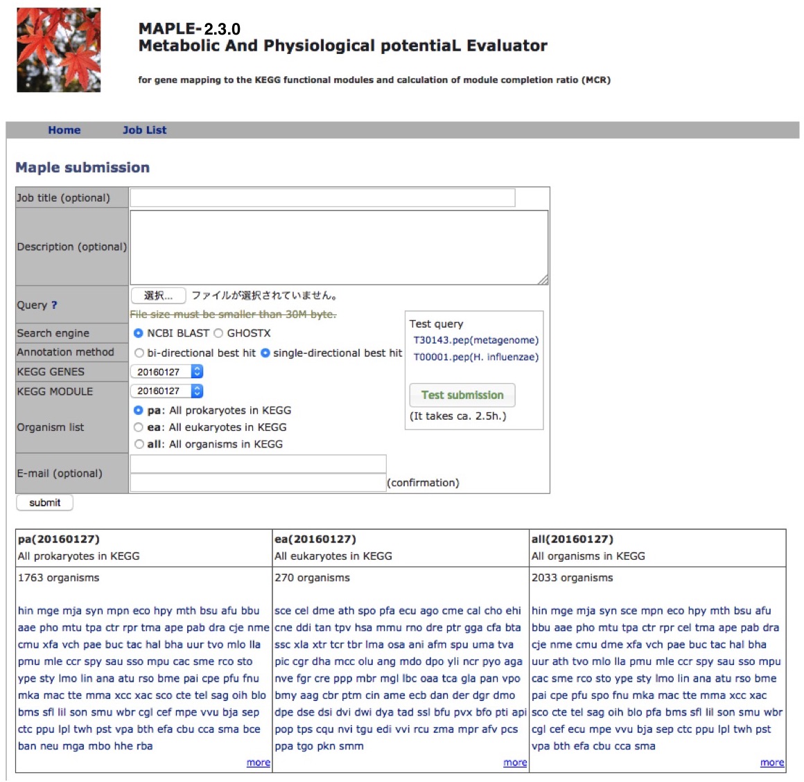
MAPLE Help

MAPLE (Metabolic And Physiological potentiaL Evaluator) is an automatic system for mapping genes in an individual genome and metagenome to a functional module and for calculating the module completion ratio (MCR) in each functional module defined by Kyoto Encyclopedia of Genes and Genomes (KEGG). First, this system assigns KEGG orthology (KO) to the query genes using the KEGG automatic-annotation server (KAAS) and maps the KO-assigned genes to the KEGG functional modules automatically. After mapping genes to modules, MAPLE automatically calculates MCR of each functional module. MAPLE can display results of comparative analyses of mapping patterns, MCR results, and abundance of completed modules not only among KEGG-annotated genomes but also among user jobs as well as between user jobs and KEGG-annotated genomes.

Data Submission

Query sequences

A metagenome
For submission of metagenomic data, query sequences must be amino acid sequences containing partial genes in metagenomic sequences generated by high-throughput DNA sequencers such as Roche 454 or Illumina MiSeq. The KO assignments are performed by KAAS on the basis of results from the BLAST or GHOSTX program. For accurate KO assignment, amino acid (aa) sequences longer than 100 aa are recommended; small proteins like ribosomal proteins shall not be applied. The query sequences should be in multi-FASTA format with unique IDs, and the gene IDs must not include a tab character. The file size of query sequences must not exceed 100 MB (~1 million sequences). When a file size exceeds this limitation, an error message will be displayed. When more sequence data are required for analysis, a user can submit several subdatasets smaller than one million sequences derived from the same metagenomic sample and then merge results from all subdatasets into one result by clicking the "Merge" button on the job list page. Computation time is proportional to the size of a dataset.

An example of a dataset: complete or incomplete genes predicted from short read sequences
>MG0001
MVKVYAPASSANMSVGFDVLGAVTPVDGALLGDVVTVEAAETFSLNNLGRFADKLPSEPR
ENIVYQCWERFCQELGKQIPVAMTLEKNSSACVAALMAMNEHCGKPLNDTRLLALMGELE
GRISGSIHYDNVAPCFLG
>MG0002
MKLYNLKDHNEQVSFAQAVTQGLGKNQGLFFPDLPEFSLTEIDEMLKLDFVTRSAKILSA
FIGDEIPQEILEERVRAAFAFPAPVVESDVGCLELFHGPTLAFKDFGGRFMAQMLTHIAG
DKPVTILTATSGDTGDTVPRFLHDGQWSPKAT
>MG0003
MKKMQSIVLALSLVLVAPMAAQAAEITLVPSVKLQIGDRDNRGYYWDGGHWRDHGWWKQH
YEWRGNRWHLHGPPPPPRHHKKAPHDHHGGHGPGQGLGAG

Organism's data selection
The user can select organism's data from three types of dataset: all prokaryotes, all eukaryotes, and all organisms for calculation of MCR depending on the purpose before submission (Figure 1).

Database selection
The user can select a KEGG genes and modules dataset from the latest to older versions. For example, for comparison of new query data with old ones (calculated by means of an old database), the user can select the same database that was used in a previous job (Figure 1).

Homology search tool selection
The user can select one of two homology search tools: BLAST and *GHOSTX (faster homology search) (Figure 1). Because the results of homology search by BLAST and GHOSTX differ from each other, the user cannot simply compare the results with the different homology search tool. *GHOSTX is a homology search tool, which can detect remote homologues like BLAST and is about 100 times faster than BLAST by using suffix arrays. (Suzuki S. et al. (2014) PLoS ONE, 9 (8): e103833)

An individual organism
Query sequences for submission to the MAPLE system must be amino acid sequences representing a set of protein-coding genes in a complete genome or partial genome of an individual organism (Figure 1). KEGG orthology (KO) assignments are performed by KAAS on the basis of results from the BLAST P program. The query sequences should be in multi-FASTA format with unique IDs, and the gene IDs must not include a tabulator. After the KO assignment to each query sequence is finished, mapping of the KO-assigned sequences to the KEGG functional modules starts, and subsequently, the module completion ratio (MCR) is calculated.

An example of a data set: complete genes
>G0001
MVKVYAPASSANMSVGFDVLGAAVTPVDGALLGDVVTVEAAETFSLNNLGRFADKLPSEP
RENIVYQCWERFCQELGKQIPVAMTLEKNMPIGSGLGSSACSVVAALMAMNEHCGKPLND
TRLLALMGELEGRISGSIHYDNVAPCFLGGMQLMIEENDIISQQVPGFDEWLWVLAYPGI
KVSTAEARAILPAQYRRQDCIAHGRHLAGFIHACYSRQPELAAKLMKDVIAEPYRERLLP
GFRQARQAVAEIGAVASGISGSGPTLFALCDKPETAQRVADWLGKNYLQNQEGFVHICRL
DTAG
>G0002
MKLYNLKDHNEQVSFAQAVTQGLGKNQGLFFPHDLPEFSLTEIDEMLKLDFVTRSAKILS
AFIGDEIPQEILEERVRAAFAFPAPVANVESDVGCLELFHGPTLAFKDFGGRFMAQMLTH
IAGDKPVTILTATSGDTGAAVAHAFYGLPNVKVVILYPRGKISPLQEKLFCTLGGNIETV
AIDGDFDACQALVKQAFDDEELKVALGLNSANSINISRLLAQICYYFEAVAQLPQETRNQ
LVVSVPSGNFGDLTAGLLAKSLGLPVKRFIAATNVNDTVPRFLHDGQWSPKATQATLSNA
MDVSQPNNWPRVEELFRRKIWQLKELGYAAVDDETTQQTMRELKELGYTSEPHAAVAYRA
LRDQLNPGEYGLFLGTAHPAKFKESVEAILGETLDLPKELAERADLPLLSHNLPADFAAL
RKLMMNHQ
>G0003
MKKMQSIVLALSLVLVAPMAAQAAEITLVPSVKLQIGDRDNRGYYWDGGHWRDHGWWKQH
YEWRGNRWHLHGPPPPPRHHKKAPHDHHGGHGPGKHHRDFDACQALVKQAFDDEELKVAL
GLNSANSINISRLLAQICYYFEDQLNPGEYGP

Notification of MAPLE job completion

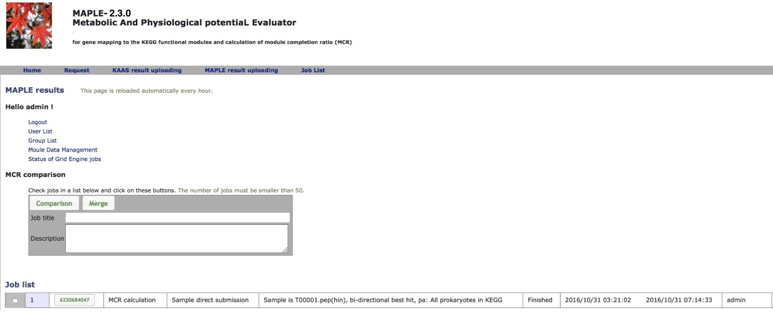
After submission of the dataset, the following message will be displayed (Figure 2): "The URL of results will be sent to the registered user's e-mail address after all processes are completed" and a job list will be present on the result page (Figure 3).

MAPLE Result Page

• An output example of MCR calculation
• An output example of comparison of multiple results

Figure 4. First picture of results corresponding to each job ID
Click to enlarge.



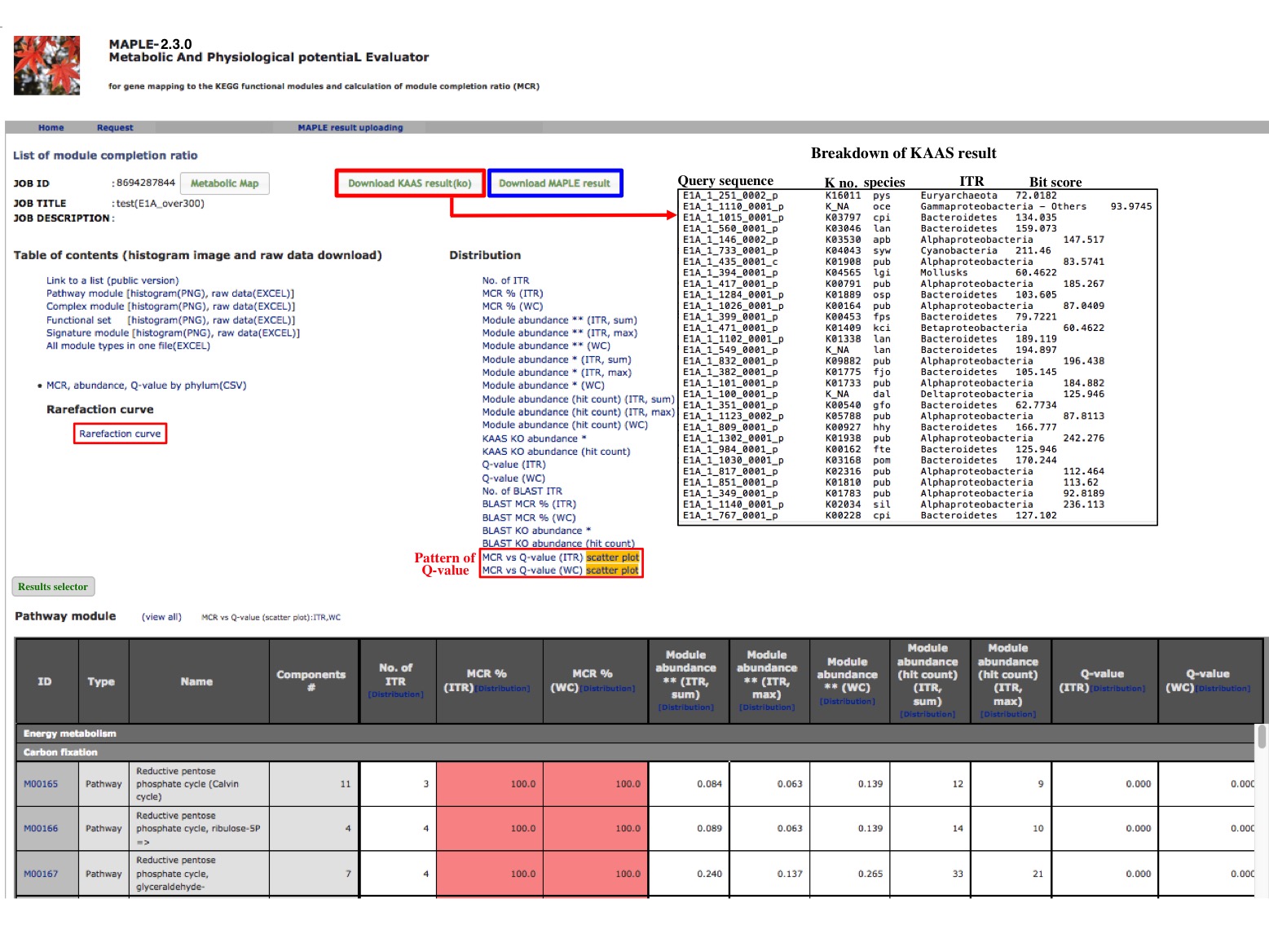
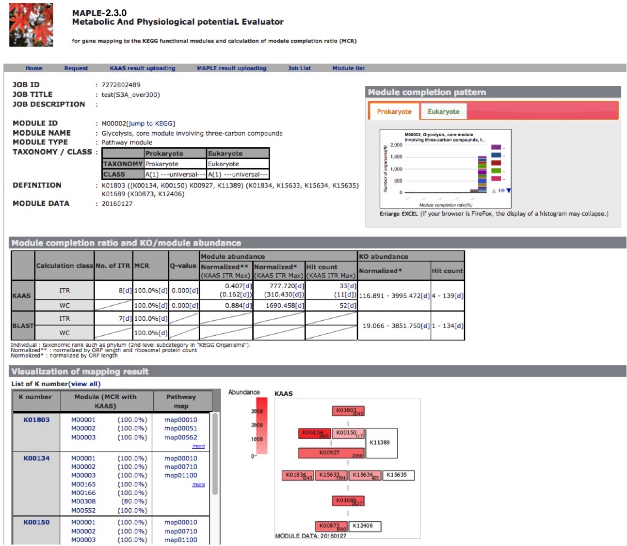
After completion of the calculation, the job ID is available for further interpretation of results (Figure 3). Clicking the job ID yields MCR (ITR for individual taxonomic rank and WC for whole community), module abundance (ITR and WC), and Q-value (ITR and WC) for determining the significance of module completeness (Figure 4). MAPLE system can yield various results by every ITR such as Gammaproteacteria, Actinobacteria, and Cyanobacteria and also by WC (whole community) (see ref. 1 for details). Users can select individual results, which appear on the result page depending on necessity from the display selector of the results (Figure 4). Users can download these data in Excel format and view all MCRs for the KEGG modules as a histogram on the first page. In addition, users can download the list of KO-assigned sequences generated by KAAS by clicking "Download KAAS results (KO)" (red rectangle). Users are advised to download the job file to reproduce all MAPLE results because each user's job will be automatically removed from the job list two weeks later. If the user clicks "Download MAPLE results" (blue rectangle), a compressed file can be downloaded. If the user uploads this file later, all MAPLE results will be reproduced on the web page. If the user clicks a module ID, the mapping pattern of the KEGG module is displayed as shown below.




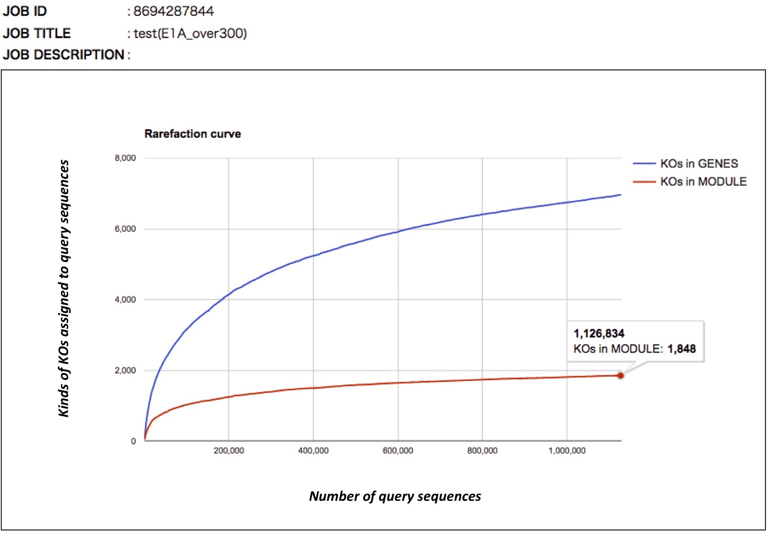
Rarefaction curve


Figure 5. Rarefaction curve to assess the richness of kinds of KOs in the metagenomic sequences.
Click to enlarge.




Rarefaction curve for assessment of richness of kinds of KOs assigned to query sequences is automatically displayed (Figure 5) by clicking "Rarefaction curve" on the results page (Figure 4).

Q-value for determining the significance of module completeness


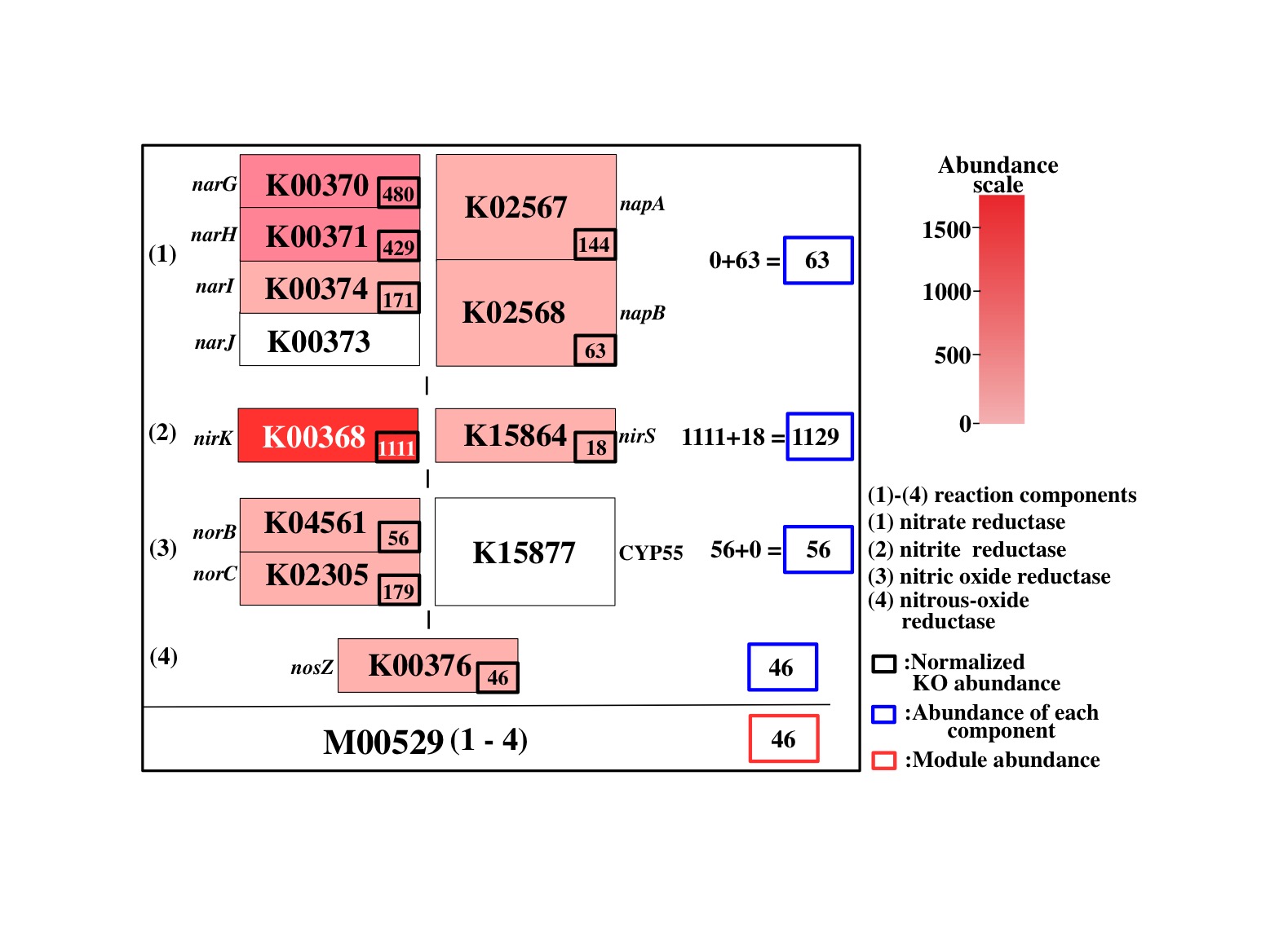
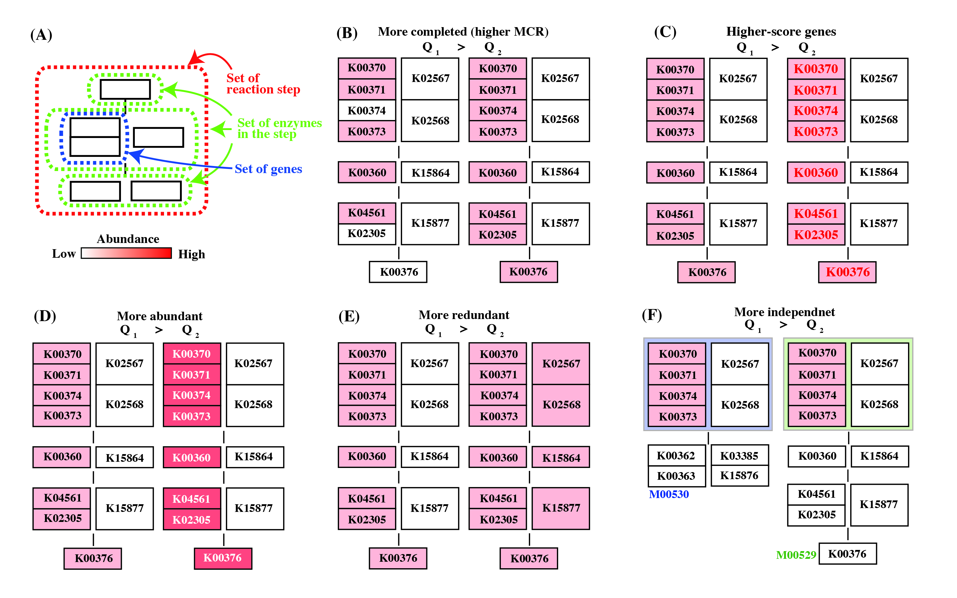Figure 6. General concept of Q-value.
Click to enlarge.
(A) Schematic diagram of reaction module. (B) - (E) As an example, the reaction module M00529 is shown. The weight of the K number (e.g., K00370) indicates the sequence similarity scores. The Q-value is lower in the following cases. (B) The module is more completed (i.e., it has a higher MCR). (C) The module consists of genes with higher similarity scores. Red numbers mean high similarity score. (D) Genes are more abundant. (E) Enzymes or reactions are alternative (e.g., isozymes exist). (F) The module is less overlapped with the other modules because of a fewer multiple comparisons. Note that the left-side module in (F) is ideal (i.e., M00529 is assumed to be independent from M00530) for the purpose of illustration.





The Q-value indicates the probability that a reaction module was identified by chance; in particular, it is calculated based on the P-values (obtained from the E-values), gene abundance, and definition of KEGG reaction modules (Figure 6A; i.e., Boolean algebra-like equations) via a multiple testing correction procedure (see Ref. 1 for details).

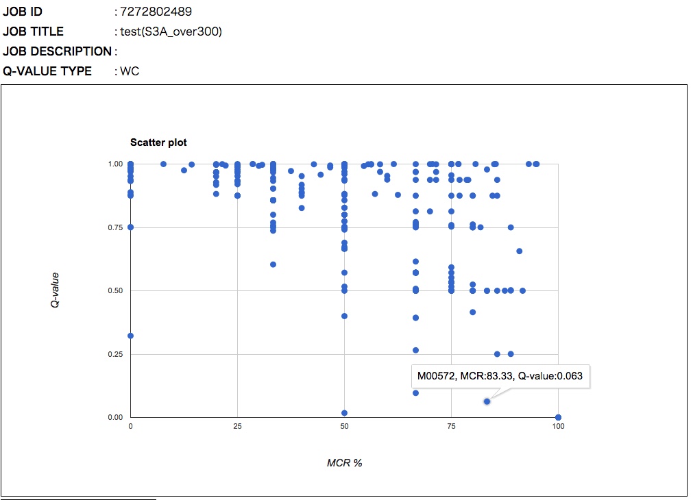
The general features of the Q-value are summarized in Figure 6. The Q-value decreases with increasing MCR and becomes smaller when genes are more abundant and when alternate reactions are available. Reaction modules that are more frequently overlapped with other modules and longer reaction modules exhibit higher Q-values because of multiple testing corrections.

According to definition of the Q-value, its value is larger than 0.5 when a straightforward (simplest or most fragile) reaction module has at least one unidentified KO (i.e., MCR < 100 %). Thus, as a criterion, we can interpret that reaction modules with Q-values of less than 0.5 are biologically feasible when the MCR is less than 100%. The patterns of Q-value to MCRs of all modules (WC and ITR) are shown in each job (Figure 7) by clicking "MCR vs Q-value" on the result page (Figure 4).


Figure 7. Pattern of Q-value to MCR of each module by WC.
Click to enlarge.




Module Completion Ratio (MCR) pattern


Figure 8. Histogram (overview) of a module completion ratio
(MCR) pattern
Click to enlarge.


When "histogram (PNG)" is clicked on the result page, the MCR patterns of each categorized module (Pathway, Complex, Functional set, and Signature) is displayed as histogram (Figure 8). And when the module name on the histogram is clicked, user can see the detailed KEGG module information and mapping pattern of the query sequences to the module (Figure 9).


Figure 9. Module information and mapping pattern to
the KEGG module
Click to enlarge.



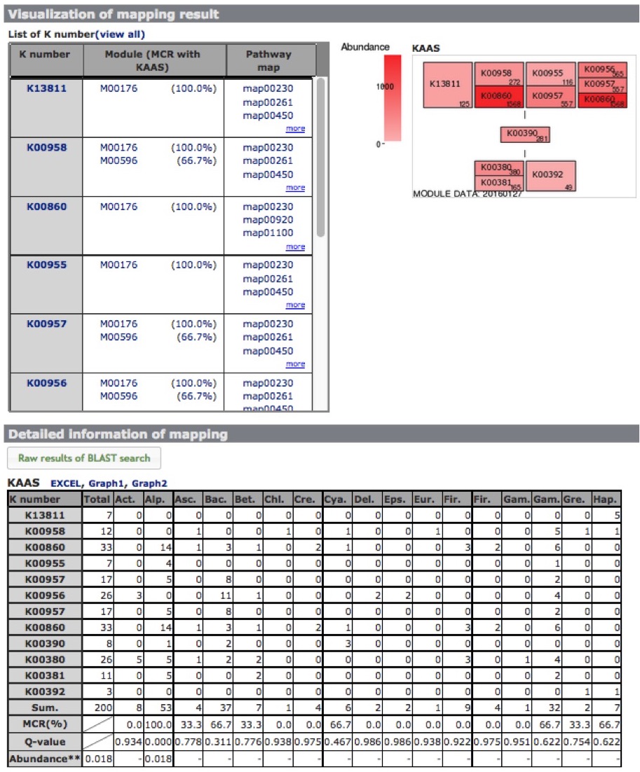
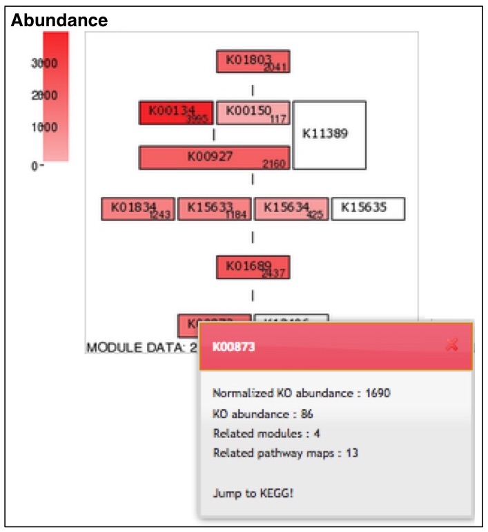
The module completion pattern of reference organisms

Distribution of MCRs in 1488 prokaryotic or 259 eukaryotic species (one genome per species) can be categorized into four patterns (universal, restricted, diversified, and nonprokaryotic/ noneukaryotic) regardless of the module type (pathway, structural complex, signature, or functional set), considering 70% of all species represent a majority measurement for patterns. Users can easily select a prokaryotic or eukaryotic pattern (Figure 9). Pattern A, defined as "universal" consists of modules completed by more than 70% of all prokaryotic or eukaryotic species. Pattern B, defined as "restricted" consists of modules completed by less than 30 % of species, with rare modules completed by less than 10% of all species. Pattern C, defined as "diversified" consists of modules ranging widely in MCR. Pattern D, defined as "nonprokaryotic" or "noneukaryotic" consists of modules that are not completed by prokaryotic or eukaryotic species (Figure 10). These four criteria and taxonomic classification for each module are helpful for interpretation of module completion patterns.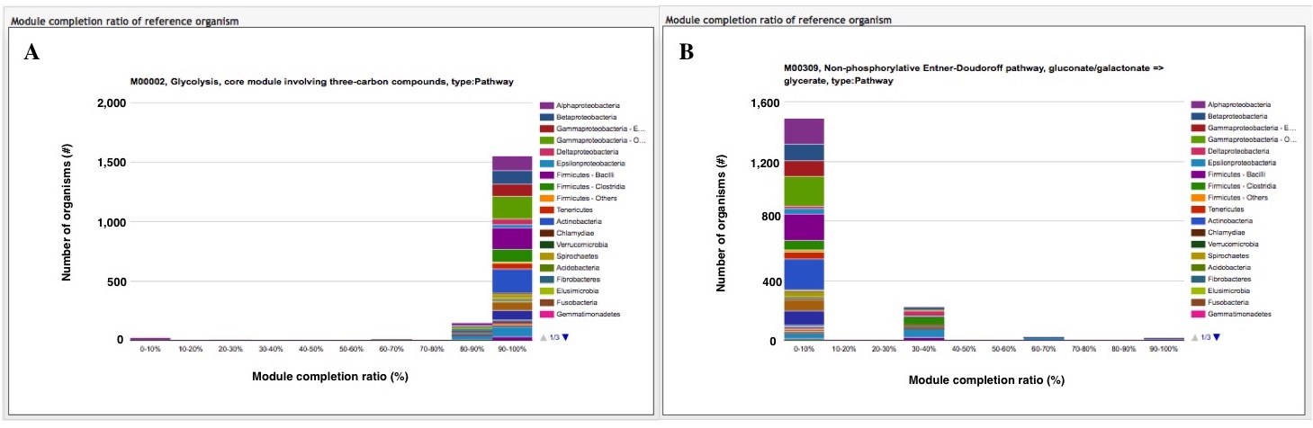


Figure 10. Module completion pattern for the KEGG modules from 1763 prokaryotic species.
Click to enlarge.
(A) The module that is completed for almost all reference organisms. (B) The module that is completed for a limited number of organisms. The breakdown of organisms for which the module is completed is color-coded by phylum level taxonomy.



The list of K numbers


Figure 11. List of K numbers and its taxonomic breakdown
Click to enlarge.



Some KO identifiers (K numbers) that are assigned to a KEGG module are shared by several other modules. These modules are listed with MCR (Figure 11). When MCR is low, the relationship between MCR of the targeted module and others assigned the same K number should be considered. In addition, all pathway maps possessing the K number assigned to the module are presented in the rightmost column. A taxonomic breakdown of sequences assigned K numbers is shown below the list of K numbers. The list from the taxonomic breakdown can be downloaded in Excel format by clicking the button "Raw results of BLAST search" (Figure 11).

The mapping pattern


Figure 12. Mapping pattern of the query sequences to the module
Click to enlarge.


KO ID-assigned sequences in the genome and metagenome are mapped to the KEGG modules. Because several sequences are assigned the same KO ID for a metagenome, IDs are mapped to the module. The abundance levels of individual KO ID-assigned sequences are differentiated by shades of red. The abundance is normalized by the average length of orthologs categorized into each KO. If the user places the cursor over a K number, detailed information on the module appears (Figure 12).

The module abundance


Figure 13. Concept of module abundance.
Click to enlarge.




The total number of sequence reads assigned to each KO constructing a module was divided by the average length of each KO group for normalization of KO abundance. This normalized KO abundance is described at the lower right corner of each KO box when the mapping pattern of the query genes to the module is displayed. The module abundance is calculated based on the normalized KO abundance. For example, the module M00529, defined as a reaction of denitrification, is composed of four reaction steps (Figure 13). In each K number set, vertically connected K numbers indicate a complex whereas horizontally located K numbers indicate alternatives. Because the enzyme responsible for the first reaction (nitrate reductase) is composed of four (left side) or two KOs (right side), unless all KOs vertically connected are filled with the KO assigned genes, the abundance of the first reaction step becomes 0. When all vertically connected KOs are filled, the minimal value of KO abundance in the vertically connected boxes becomes the abundance at the first step. Thus, the abundance of the first step in module M00529 is 63. As the second step, when two horizontally located KOs are filled with the KO assigned genes, the abundance becomes 1,129, which is sum of both KOs. The abundance at the third step becomes 56 in a similar manner as the first step, and that of the last step is 46 (Figure 13). Because the module abundance becomes the minimal value among all steps, the abundance of module M00529 is calculated to be 46.

When we compare the module abundances with those of other metagenomic samples, each sample should be normalized because the number of cells used to construct the metagenome is different depending on the sample, even if the number of sequence reads applied to MAPLE is the same. The ribosome is basically composed of the same number of ribosomal proteins, regardless of the species, although some species possesses accessory proteins and almost all genes encoding ribosomal proteins are single copy, i.e., the number of ribosomal proteins in the metagenome reflects number of cells. In MAPLE system, we calculated the module abundance per ribosomal protein to facilitate the comparison between the different environmental sites (see Ref. 1 for details).



Virtual module for ribosome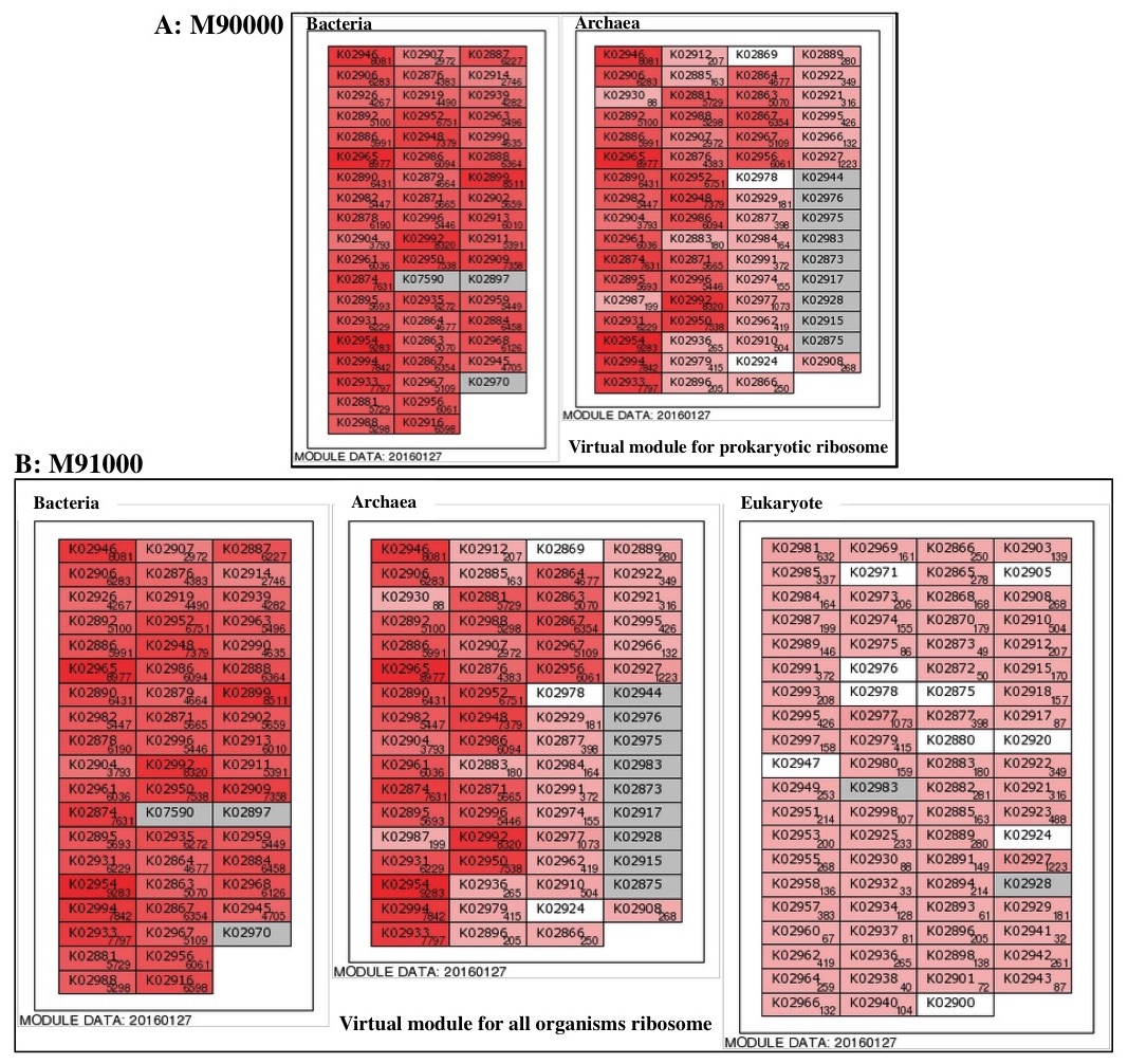
(M90000 for prokaryote & M91000 for all organisms)


Figure 14. Virtual ribosome modules for taxonomic analysis
in the metagenome.
Click to enlarge. A: M90000 (virtual prokaryotic module),
B: M91000 (virtual module for all organisms)




Ribosomal proteins are well conserved among all organisms and possess sequences specific to each individual organism; therefore, ribosomal proteins can be used for identification of organisms (see Ref. 1 for details). User can perform taxonomic analysis and calculate the ratio of bacteria and archaea (M90000 for prokaryote), and also that of bacteria, archaea and eukaryote (M91000 for all organisms) in the metagenome using virtual ribosome modules included in MAPLE system (Figure 14). However, the calculated results such as MCR, Q-value, and module abundance for the virtual modules do not make sense. Because the archaeal ribosome, which contains 58 ribosomal proteins, has six more proteins than the bacterial ribosome, user should normalize the total number of archaeal ribosomal proteins to the number of bacterial ribosomal proteins by multiplying by 52/58. Similar to archaea, since the eukaryotic ribosome contains 77 ribosomal proteins, user should normalize by multiplying by 52/77 and users can sum up the number of bacterial ribosomes and normalized archaeal and eukaryotic ribosomes and then use this sum as a denominator to calculate the ratio of archaea, eukaryote and bacteria. Users can also calculate the ratio of each taxonomic level defined by KEGG, such as phylum and class, in the metagenome using the same manner.

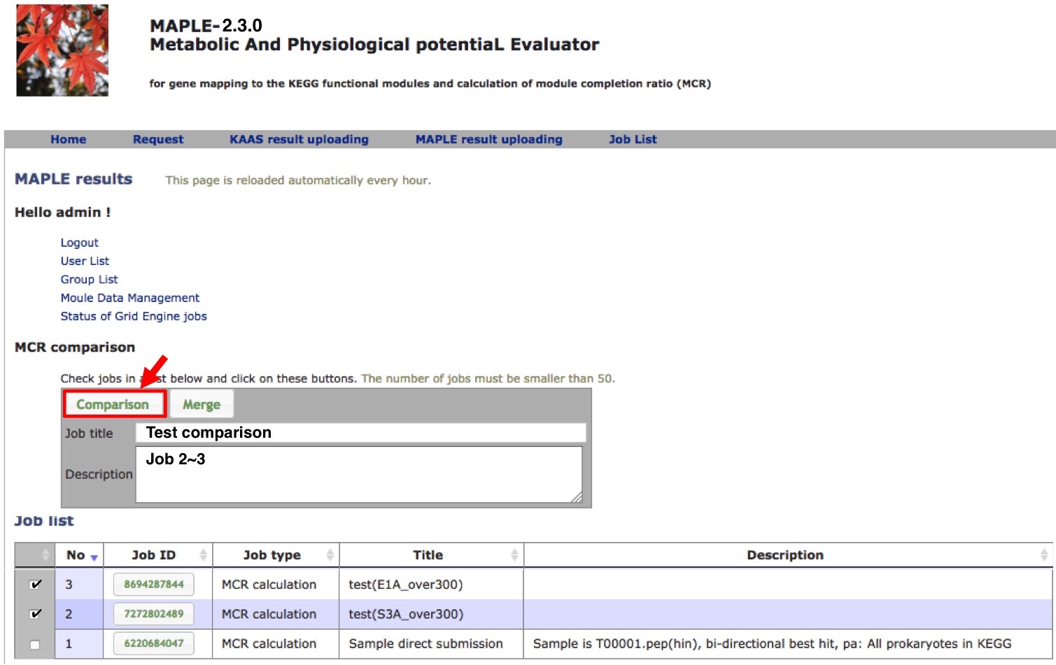
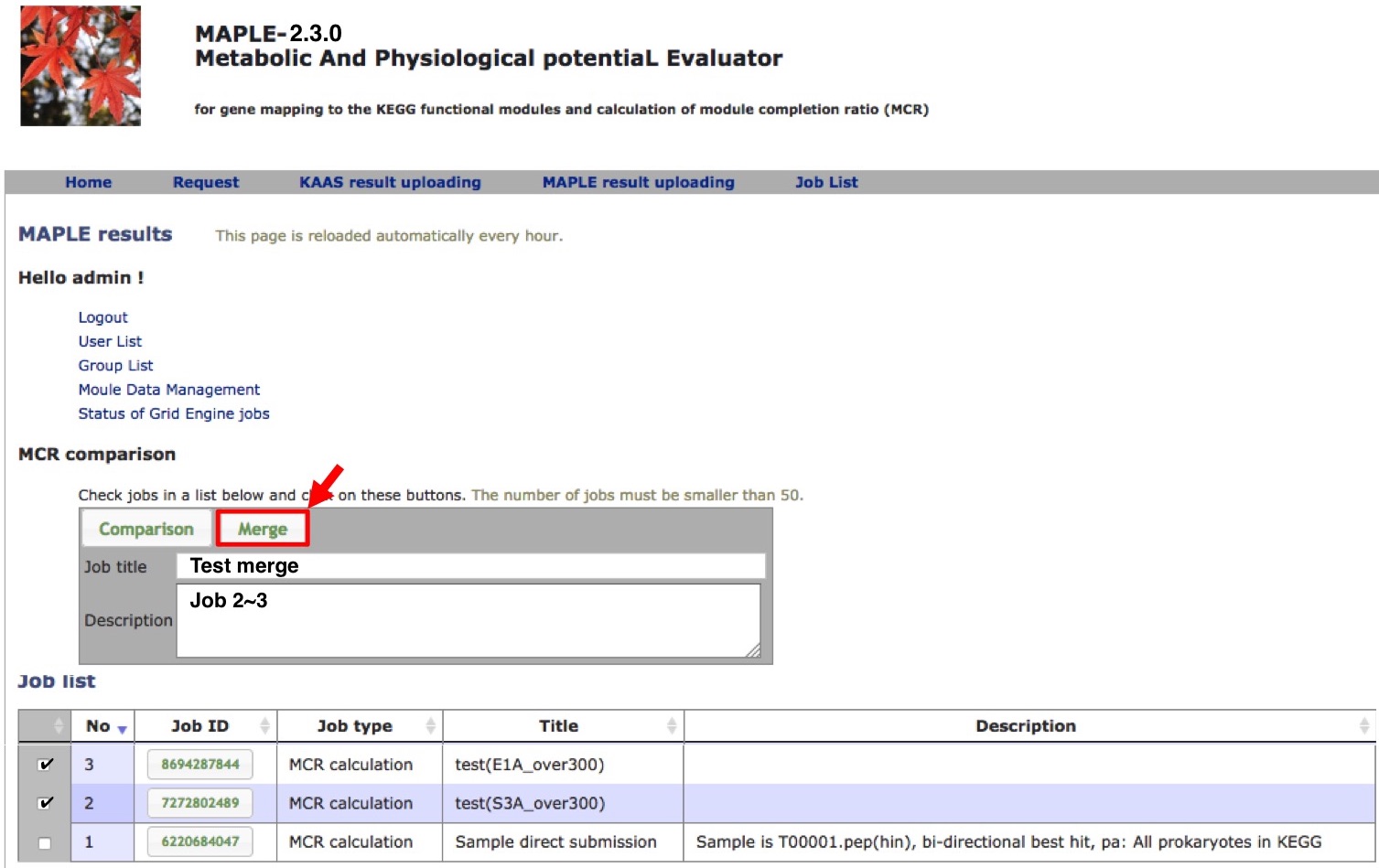
Comparison of multiple results


Figure 15. User's customized job list
Click to enlarge.

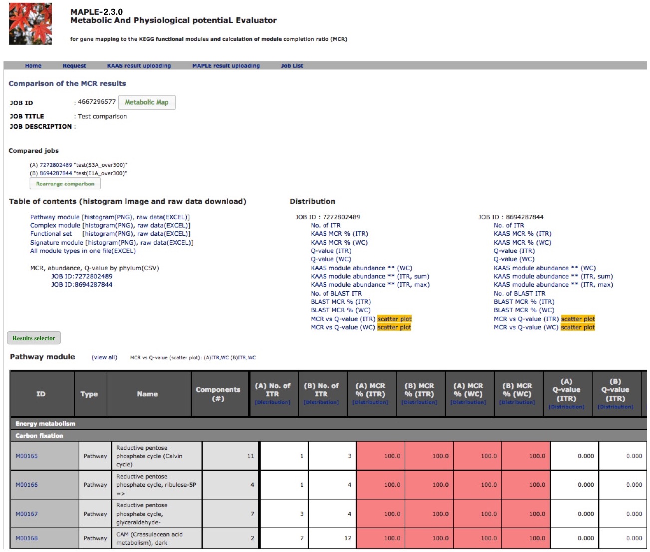
Comparison of several custom jobs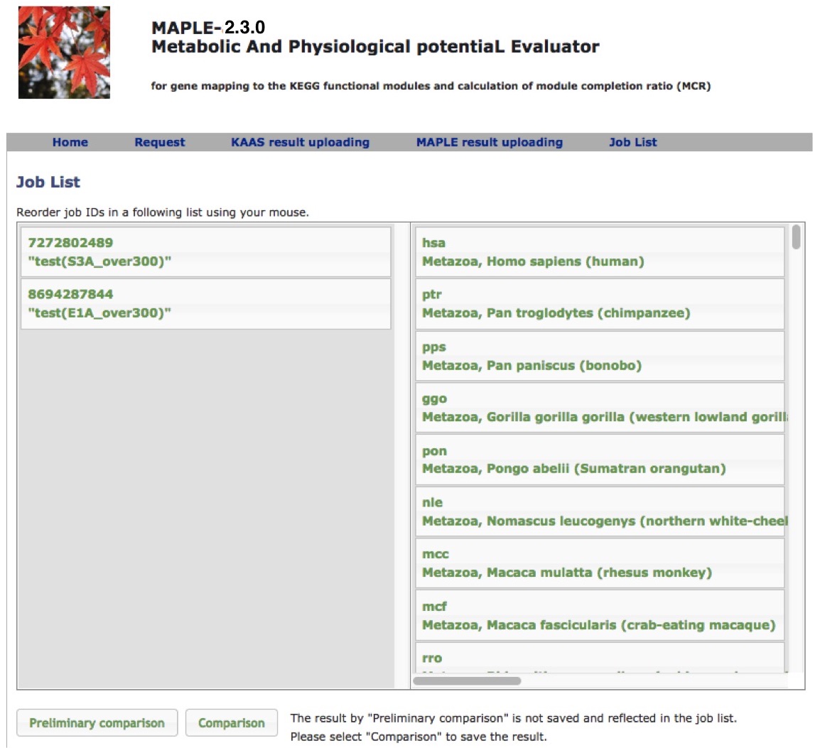
When several IDs of jobs to be compared are checked in the job list (Figure 15) and the "Comparison" button is pressed, the job arrangement page will be displayed (Figure 16). The user can add preanalyzed individual organisms from the organism list if necessary and change their displayed order.





Figure 16. Job arrangement page for comparative analysis
Click to enlarge.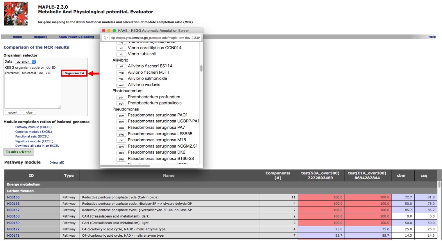

Figure 17. Results of the preliminary comparison
Click to enlarge.

Preliminary comparison
When users want to compare their own job results or results from preanalyzed individual organisms, they may select organisms to be compared from the organism list. If it is not necessary to save results of the preliminary study, please select "Preliminary comparison" on the job arrangement page (Figure 16) to view comparative results. When users want to include additional preanalyzed individual organisms or to delete them, they can select organisms to be added for comparison from the pull-down menu of the organism list or delete an unnecessary organism (Figure 17).





Figure 18. Comparison results from two custom jobs
Click to enlarge.

Comparison and saving results
When the combination and order of user job IDs and preanalyzed organisms to be compared are fixed in a preliminary comparison, users can select "Comparison" to display and save the final comparative results. The saved results will be reflected in the user job list as a new job. The comparison results will be displayed as shown in Figure 18. If necessary, users can rearrange comparison even at this stage. If the user clicks "Rearrange comparison" (red rectangle), he/she will be taken to the job arrangement page (Figure 16).





Figure 19. Merging the MAPLE results from two subdatasets
Click to enlarge.

Merging results of subdatasets
Because the file size of query sequences must not exceed 100 MB (approximately 1 million sequences), the user can submit several subdatasets smaller than one million sequences several times, if more sequence data are necessary for analysis. Then, several results from subdatasets can be merged and displayed as one result by using the "Merge" function (Figure 19). Users can select the job IDs to be merged from the job list and view the merged results by clicking the "Merge" button (red rectangle). When two jobs with 1 million sequences are merged as one job, it will take approximately 5 hours.





Figure 20. Uploading the job file to reproduce previous
MAPLE results
Click to enlarge.

Uploading MAPLE results
As mentioned above, users are advised to download the compressed job file on the result page to preserve all MAPLE results (Figure 4) because each user job file will be automatically removed from the job list 2 weeks later. If the user uploads this file later to the homepage of MAPLE, all MAPLE results will be reproduced on the web page (Figure 20).